The Gyroscope and the Tippe Top

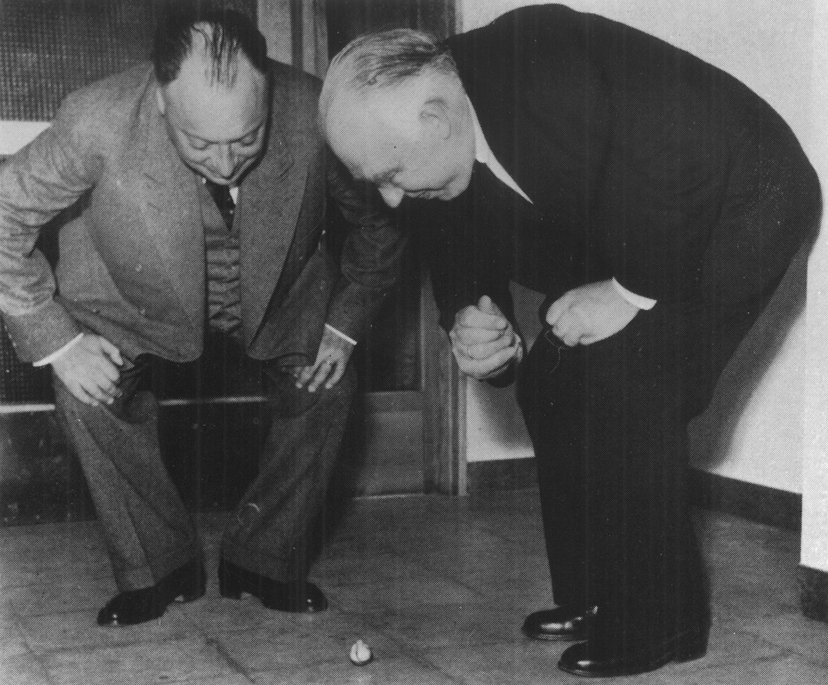
The photograph is one of the most reproduced in the history of physics. Two of the greatest physicists of the twentieth century stand bent forward, hands on knees, watching a toy with the same concentration they otherwise gave to quantum mechanics.

The toy had been patented as early as 1891 by Helene Sperl in Munich, but the patent lapsed the following year. The engineer Werner Østberg reinvented it in 1950 after a journey in South America, where he had seen people spin a small round fruit by its stalk. The fruit turned over and carried on spinning on its stalk. Østberg called his top the ‘tippetop’, mass-produced it and took out patents in several countries. Within a few years it was sold all over the world – in Canada for 25 cents at the chemist's, and in the USA in cereal boxes.

Bohr was delighted. According to the Danish newspaper Politiken of 1 June 1951, he showed the top to the King of Sweden at the inauguration in Lund. The puzzle was discussed in the daily press, and in 1952 the first theoretical papers appeared, among them by C. M. Braams and N. M. Hugenholtz in Physica. J. L. Synge at first thought that friction was irrelevant, but was persuaded by the others. For friction is the whole key, as the simulation above and the theory below show.

The gyroscope

The vector picture

If the rotor spins fast, $\mathbf L\approx I_3\omega_3\,\hat{\mathbf e}_3$. The torque of gravity about the pivot is $\boldsymbol\tau = l\,\hat{\mathbf e}_3\times(-Mg\,\hat{\mathbf z})$. It is horizontal and perpendicular to $\mathbf L$, so only the direction changes:

$$\dot{\hat{\mathbf e}}_3=\boldsymbol\Omega\times\hat{\mathbf e}_3,\qquad \Omega=\frac{Mgl}{I_3\,\omega_3}.$$

The faster the rotor spins, the more slowly the axle precesses. These are the orange and the blue vectors in the simulation: $\boldsymbol\tau$ always points where $\mathbf L$ is heading.

The Lagrangian and the conserved quantities

With the Euler angles $\theta$ (tilt), $\phi$ (precession) and $\psi$ (spin),

$$\mathcal L=\tfrac12 I_1\left(\dot\theta^2+\dot\phi^2\sin^2\theta\right)+\tfrac12 I_3\left(\dot\psi+\dot\phi\cos\theta\right)^2-Mgl\cos\theta .$$

$\phi$ and $\psi$ are cyclic, so two angular momenta are conserved together with the energy:

$$L_3=I_3\left(\dot\psi+\dot\phi\cos\theta\right)=I_3\omega_3,\qquad L_z=I_1\dot\phi\sin^2\theta+L_3\cos\theta .$$

Steady precession

The Lagrange equation for $\theta$ is $I_1\ddot\theta=I_1\dot\phi^2\sin\theta\cos\theta-L_3\dot\phi\sin\theta+Mgl\sin\theta$. Setting $\ddot\theta=\dot\theta=0$ gives a quadratic in $\dot\phi$:

$$I_1\cos\theta\,\dot\phi^2-L_3\dot\phi+Mgl=0\quad\Longrightarrow\quad \dot\phi=\frac{2Mgl}{L_3\pm\sqrt{L_3^2-4I_1Mgl\cos\theta}}.$$

For a fast top the plus sign gives the slow branch $\dot\phi\approx Mgl/(I_3\omega_3)$, and the minus sign the fast one $\dot\phi\approx I_3\omega_3/(I_1\cos\theta)$. The button Steady precession starts the gyroscope exactly on the slow branch.

Nutation: why the axle traces arcs when released from rest

Eliminate $\dot\phi$ and $\dot\psi$ using the conserved quantities. The $\theta$ motion then becomes one-dimensional in an effective potential:

$$E'=\tfrac12 I_1\dot\theta^2+\frac{\left(L_z-L_3\cos\theta\right)^2}{2I_1\sin^2\theta}+Mgl\cos\theta .$$

$\theta$ oscillates between two turning points. If the axle is released from rest, $\dot\phi=0$ at the upper turning point and the trail has sharp corners (cycloid-like arcs). For a fast top the nutation frequency is roughly $I_3\omega_3/I_1$, and the amplitude falls off as $1/\omega_3^2$. Turn up the spin rate in the simulation and watch the arcs shrink.

Friction in the bearing: why the gyroscope eventually sinks

A torque along the axle, $\dot L_3=-kL_3$, reduces $L_3$. Since the precession goes as $1/L_3$, it gets faster and faster, and the axle sinks. In the simulation the gyroscope stops when the rotor hits the tower.

The tippe top

Geometry

The ball has radius $R$ and centre $O$. The centre of mass $C$ lies $\alpha R$ from $O$ along the axis of symmetry, and $\hat{\mathbf e}_3$ points from $C$ towards the stem. $\theta=0$ is the top on its ball, $\theta=\pi$ on its stem. The contact point $P$ always lies directly below $O$, so

$$\mathbf a=\overrightarrow{CP}=R\left(\alpha\hat{\mathbf e}_3-\hat{\mathbf z}\right),\qquad z_C=R\left(1-\alpha\cos\theta\right).$$

A full inversion raises the centre of mass by $2\alpha R$.

Equations of motion and energy loss

The force from the table, $\mathbf F=N\hat{\mathbf z}+\mathbf F_f$, acts at $P$:

$$M\dot{\mathbf v}_C=\mathbf F-Mg\hat{\mathbf z},\qquad \dot{\mathbf L}=\mathbf a\times\mathbf F,\qquad \mathbf F_f=-\mu N\frac{\mathbf v_P}{|\mathbf v_P|}.$$

The slip velocity $\mathbf v_P=\mathbf v_C+\boldsymbol\omega\times\mathbf a$ is horizontal, so the normal force does no work, and $\dot E=\mathbf F_f\cdot\mathbf v_P\le 0$. The simulation solves exactly these equations, with the normal force fixed by the requirement that the ball stays on the table.

Jellett's constant

Put $J=\mathbf L\cdot\mathbf a$. Then $\dot J=(\mathbf a\times\mathbf F)\cdot\mathbf a+\mathbf L\cdot\dot{\mathbf a}$. The first term is zero. With $\dot{\mathbf a}=\alpha R\,\boldsymbol\omega\times\hat{\mathbf e}_3$ and $\mathbf L=I_1\boldsymbol\omega+(I_3-I_1)\omega_3\hat{\mathbf e}_3$, both triple products contain two identical vectors:

$$\dot J=\alpha R\left[I_1\,\boldsymbol\omega\cdot(\boldsymbol\omega\times\hat{\mathbf e}_3)+(I_3-I_1)\,\omega_3\,\hat{\mathbf e}_3\cdot(\boldsymbol\omega\times\hat{\mathbf e}_3)\right]=0 .$$

So $J=R(\alpha L_3-L_z)$ is conserved exactly, whatever the friction law. It is the flat green line in the graph above.

Final spin and the energy threshold

Start with $\omega_0$ at $\theta=0$ and finish with $\omega_1$ at $\theta=\pi$. Conservation of $J$ gives

$$I_3\omega_0(\alpha-1)=-I_3\omega_1(1+\alpha)\quad\Longrightarrow\quad \omega_1=\frac{1-\alpha}{1+\alpha}\,\omega_0 .$$

Seen from the table the top spins the same way, but relative to the body the rotation has reversed. Since friction can only remove energy, the inversion requires $E_1\le E_0$, and with $1-\left(\frac{1-\alpha}{1+\alpha}\right)^2=\frac{4\alpha}{(1+\alpha)^2}$ this reduces to

$$\omega_0^2\ge\frac{MgR\,(1+\alpha)^2}{I_3}.$$

Stability: the energy landscape

For fast spin the rotational energy dominates. Minimise $\tfrac12\mathbf L\cdot I^{-1}\mathbf L$ subject to the constraint $\mathbf L\cdot\mathbf a=J$. The Lagrange multiplier gives $\boldsymbol\omega=\lambda\mathbf a$: the top rotates about the line $CP$, and the contact point does not slip. The energy is then

$$E_{\rm rot,min}(\theta)=\frac{J^2}{2R^2f(\theta)},\qquad f(\theta)=I_1\sin^2\theta+I_3(\alpha-\cos\theta)^2,$$ $$f'(\theta)=2\sin\theta\left[(I_1-I_3)\cos\theta+\alpha I_3\right].$$

The upright state is an energy minimum precisely when $I_1/I_3 \lt 1-\alpha$. The inverted state is a minimum precisely when $I_1/I_3 \lt 1+\alpha$. The top therefore inverts when

$$1-\alpha \lt \frac{I_1}{I_3} \lt 1+\alpha .$$

For $I_1/I_3 \gt 1+\alpha$ it ends in a tilted, precessing state with $\cos\theta^*=\alpha I_3/(I_3-I_1)$. Friction draws energy out at fixed $J$, and the top rolls down the landscape, exactly as the dot in the graph shows.

The boiled egg: the same physics as the tippe top

The boiled egg is a rigid body sliding on the table, just like the tippe top. The contact point slips, friction removes energy, and the quantity $J=\mathbf L\cdot\mathbf a$ is approximately conserved – exactly for a sphere, only approximately for an egg. In 2002 Keith Moffatt and Yutaka Shimomura gave the full explanation of how the egg rises in a slow ‘gyroscopic balance’.

Think of the egg as an elongated ellipsoid of revolution with semi-axes $a>b$ and the moments of inertia $I_1=\tfrac15M(a^2+b^2)$ about a transverse axis and $I_3=\tfrac25Mb^2$ about the long axis. Lying down, $|\mathbf a|=b$; standing, $|\mathbf a|=a$. At fixed $J$, $L=J/|\mathbf a|$, so

$$E_{\text{lying}}=\frac{J^2}{2I_1b^2},\qquad E_{\text{standing}}=\frac{J^2}{2I_3a^2},\qquad \frac{E_{\text{standing}}}{E_{\text{lying}}}=\frac{a^2+b^2}{2a^2}<1 .$$

The standing egg has the lower rotational energy, and friction takes it there. In return, the centre of mass is raised by $a-b$. With $a=3$ cm and $b=2.2$ cm the energy ratio is 0.77, and the requirement $(1-0.77)\tfrac12I_1\omega^2\ge Mg(a-b)$ gives $\omega\gtrsim50$ rad/s, about 8 revolutions per second.

Which end does it stand on?

A real egg has a broad and a pointed end, and the centre of mass lies nearer the broad one. The egg can stand up on either end. Kenzo Sasaki showed in 2004 that it depends on the egg's shape and on how it is tilted at the start: there is a critical angle, and if the starting angle lies on one side of it the egg stands up on its pointed end, otherwise on its broad end. According to Sasaki the egg most often ends on its broad end, but it can also stand on its pointed end with the broad end up – and then it resembles the tippe top, ending with its centre of mass as high as possible. Try it yourself with several eggs. In the simulation you choose with the initial tilt $\theta_0$.

The raw egg: the liquid lags behind

In a raw egg only the shell is rigid. White and yolk are a liquid, coupled to the shell only through viscosity. Treating the shell as a thin spherical shell with a tenth of the mass, and the contents as a solid sphere, $I_{\text{shell}}/I_{\text{liquid}}=\tfrac23m_{\text{shell}}r^2\big/\tfrac25m_{\text{liquid}}r^2\approx0.19$.

When you twist the egg into motion, the shell gets the angular velocity $\omega_0$ while the liquid stays still. Soon they share the angular momentum and end with

$$\omega=\frac{I_{\text{shell}}}{I_{\text{shell}}+I_{\text{liquid}}}\,\omega_0\approx0.16\,\omega_0 .$$

The raw egg spins at only a sixth of the speed, and 84% of the energy has gone into viscous friction in the liquid. It never reaches the 8 revolutions per second – and in any case the liquid would not follow like a rigid body if the egg began to tip.

If you stop the shell with a finger, you brake only the shell. The liquid carries on, as Newton's first law demands, and when you let go it hands back its angular momentum: the egg turns again at about $0.84\,\omega_{\text{liquid}}$. A boiled egg has no hidden rotation and stays put. This is the classic way to tell a boiled egg from a raw one without breaking it.

The principle: integrate twice

If you know the starting point and the starting velocity, the acceleration gives the rest: $\mathbf v(t)=\mathbf v_0+\int_0^t\mathbf a\,dt$ and $\mathbf r(t)=\mathbf r_0+\int_0^t\mathbf v\,dt$. It sounds simple, but two things make it hard.

First, an accelerometer does not measure the acceleration $\mathbf a$. It measures the specific force $\mathbf f=\mathbf a-\mathbf g$, the force per unit mass from everything except gravity. An accelerometer lying still on the table reads $9.81\ \mathrm{m/s^2}$ upwards, and one in free fall reads zero. The navigation computer has to add gravity back itself:

$$\ddot{\mathbf r}=\mathbf f+\mathbf g(\mathbf r).$$

Second, $\mathbf f$ is measured along the instrument's own axes, and you must know precisely how these are oriented relative to the vertical and to north. If the instrument is tilted by a small angle $\delta$, part of gravity, $g\,\delta$, is read as a horizontal acceleration. An error of one milliradian (0.06°) gives $0.01\ \mathrm{m/s^2}$, and after an hour the position has overshot by $\tfrac12\cdot 0.0098\cdot 3600^2\approx 64$ km.

Keeping the direction is the gyroscope's job. With no torque, $\dot{\mathbf L}=\mathbf 0$, so a fast rotor holds its axis fixed relative to the fixed stars, however the vehicle turns around it. It is the same $\dot{\mathbf L}=\boldsymbol\tau$ as in the simulation at the top, only with $\boldsymbol\tau$ made as small as it can possibly be. The bearing friction that makes the gyroscope above sink is exactly the kind of error designers have fought against for a hundred years.

On the rotating Earth two fictitious terms come in. In an Earth-fixed frame with the Earth's angular velocity $\boldsymbol\Omega_\oplus$,

$$\ddot{\mathbf r}=\mathbf f-2\boldsymbol\Omega_\oplus\times\dot{\mathbf r}+\mathbf g_{\rm eff}(\mathbf r),$$

where $\mathbf g_{\rm eff}$ includes the centrifugal term. The Coriolis term is the same one that turns Foucault's pendulum.

Two designs: stable platform and strapdown

The gimballed platform

In the classical systems three gyroscopes and three accelerometers sit on a small platform hung in gimbals. When the vehicle turns, the gyroscopes sense it and servo motors turn the gimbals back, so that the platform stays level and pointing north. The accelerometers then measure directly north, east and vertical, and the computer only has to integrate.

Three gimbals have one weakness: gimbal lock. When the middle gimbal has turned through 90°, the inner and outer axes line up, and one degree of freedom disappears. It is the same singularity seen in the gyroscope's equations above, where $\sin^2\theta$ stands in the denominator of the equation for $\ddot\phi$: Euler angles cannot describe every orientation smoothly. The platform in the Apollo spacecraft had only three gimbals, and the astronauts had to steer clear of the dangerous orientations. During Apollo 11 Michael Collins jokingly asked for a fourth gimbal for Christmas.

Strapdown

In modern systems the sensors are bolted to the vehicle. The gyroscopes measure the angular velocity $\boldsymbol\omega$ in the vehicle's own axes, and the computer keeps track of the orientation, typically as a quaternion $q$:

$$\dot q=\tfrac12\,q\otimes(0,\boldsymbol\omega).$$

The accelerometer readings are then rotated into a north–east–down frame with $q$ before integration. Quaternions have no singularity, so gimbal lock disappears. In return the computer must calculate hundreds of times a second, and the sensors must be able to follow the vehicle's fastest turns. That is why strapdown only broke through in the 1980s, when the computing power and a new kind of gyroscope were in place.

Gyroscopes without a spinning top

The ring laser and the Sagnac effect

Two laser beams run in opposite directions round a closed light path. When the instrument is at rest, the two paths are equally long. If it turns with angular velocity $\Omega$ about an axis perpendicular to the light path, the path going with the rotation becomes longer and the one going against it shorter. In a ring laser this gives a frequency difference

$$\Delta f=\frac{4A}{\lambda P}\,\Omega ,$$

where $A$ is the enclosed area and $P$ the perimeter. A triangular cavity with 10 cm sides and a helium–neon laser ($\lambda=633$ nm) gives, at the Earth's rotation of $7.29\cdot10^{-5}$ rad/s, a difference of about 7 Hz between two frequencies of $4.7\cdot10^{14}$ Hz. At very slow rotation the two waves lock onto each other. This is overcome by shaking the whole block slightly back and forth. The great advantage of the ring laser is that nothing rotates and nothing wears.

Fibre-optic and vibrating gyroscopes

The fibre-optic gyroscope sends the light many times round a coil of optical fibre. The phase difference is $\Delta\varphi=8\pi NA\,\Omega/(\lambda c)$ for $N$ turns, so a long fibre gives high sensitivity.

The gyroscope in a mobile phone is a MEMS structure: a tiny silicon mass vibrating back and forth with velocity $\mathbf v$. When the chip turns, the Coriolis force $-2m\,\boldsymbol\Omega\times\mathbf v$ acts perpendicular to the vibration and sets off a second oscillation, which is measured capacitively. These are two coupled oscillations, with the rotation as the coupling. A related principle is used in the very precise hemispherical resonators: G. H. Bryan noticed in 1890 that the vibration pattern of a ringing wine glass that is turned does not quite turn with the glass.

Schuler: a pendulum as long as the Earth's radius

A platform that is to be kept level on a sphere cannot simply be held fixed in inertial space. When the vehicle moves a distance $x$ northwards, the plumb line has turned through the angle $x/R$. The platform must therefore be turned at the angular velocity $v/R$, calculated from the speed the system has itself worked out.

Max Schuler, cousin of the gyrocompass inventor Hermann Anschütz-Kaempfe, showed in 1923 that this makes the system self-correcting. If the calculated speed is too high, the platform is turned too far and tilts. Part of gravity is then read as a deceleration, which pulls the speed error back. With the tilt error $\psi$, the speed error $\delta v$, a constant accelerometer bias $b$ and a constant gyro drift $\varepsilon$,

$$\delta\dot v=-g\,\psi+b,\qquad \dot\psi=\frac{\delta v}{R}+\varepsilon\qquad\Longrightarrow\qquad \delta\ddot x=-\frac gR\,\delta x+b-g\,\varepsilon\,t .$$

The left-hand side and the first term on the right are the equation of a pendulum of length $R$. The period is

$$T_S=2\pi\sqrt{\frac Rg}=84.4\ \text{min},$$

the same orbital period as a satellite circling just above the Earth's surface. Starting from rest, the solutions are

$$\delta x_b=\frac{bR}{g}\left(1-\cos\omega_S t\right),\qquad \delta x_\varepsilon=-R\,\varepsilon\left(t-\frac{\sin\omega_S t}{\omega_S}\right),\qquad \omega_S=\sqrt{g/R}.$$

An accelerometer error gives only a bounded oscillation. An error of 100 µg ($10^{-4}g$) makes the position swing between 0 and 1.3 km. Without Schuler tuning the same error would give $\tfrac12bt^2$: 6.4 km after one hour and 230 km after six. Gyro drift is worse, because it gives an error that grows steadily with time. A drift of 0.01°/h gives $R\varepsilon\approx 1.1$ km/h, or roughly 0.6 nautical miles an hour. That is why the accuracy of navigation systems is quoted in nautical miles per hour.

The vertical has no such rescue. Gravity decreases with height, so too large a calculated height gives too small a calculated gravity, and the error grows: $\delta\ddot h=+(2g/R)\,\delta h$, with the time constant $\sqrt{R/2g}\approx 9.5$ min. Height is therefore always supported by a barometric altimeter.

From Foucault to the mobile phone

In 1852 Léon Foucault gave the gyroscope its name: he wanted to see the rotation of the Earth with a rotor that held its direction while the laboratory turned beneath it. In 1908 Hermann Anschütz-Kaempfe built the first usable gyrocompass, because he wanted to take a submarine to the North Pole, and Schuler's analysis of 1923 turned it into a navigation instrument that could cope with a ship's motion.

The V-2 rocket of 1944 held its heading with gyroscopes and cut its engine when an integrating accelerometer had counted up to the right speed. In 1953 Charles Stark Draper of MIT flew an aircraft from Massachusetts to Los Angeles with an inertial system and no navigator. In 1958 the submarine USS Nautilus sailed under the North Pole with an inertial system on board. There both the old compasses were useless: the magnetic compass because the field lines stand almost vertical that far north, and the gyrocompass because the Earth's axis of rotation is vertical at the pole, so there is no horizontal component to settle towards.

Today ring-laser gyroscopes sit in strapdown systems in every large airliner, and MEMS gyroscopes in phones, cars and drones. Satellite navigation and inertial navigation complement each other, typically coupled in a Kalman filter: the satellites keep the drift down over long periods, and the inertial system covers the seconds and minutes when the signal is missing. An inertial system can be neither shadowed nor jammed from outside, and it has become topical again since GPS interference has in recent years affected air traffic over the Baltic.

The oscillation of the position error with its period of 84.4 minutes is a pendulum without coupling. Oscillations that exchange energy with one another are the subject of the page on coupled pendulums.

The full derivation with figures is available as a report (in Danish):

References

• H. Goldstein, C. Poole & J. Safko, Classical Mechanics, 3rd ed., Addison-Wesley (2002), ch. 5.
• J. H. Jellett, A Treatise on the Theory of Friction, Dublin (1872).
• C. M. Braams, ‘On the influence of friction on the motion of a top’, Physica 18, 503 (1952).
• N. M. Hugenholtz, ‘On tops rising by friction’, Physica 18, 515 (1952).
• R. J. Cohen, ‘The tippe top revisited’, Am. J. Phys. 45, 12 (1977).
• S. Ebenfeld & F. Scheck, ‘A new analysis of the tippe top’, Ann. Phys. 243, 195 (1995).
• N. M. Bou-Rabee, J. E. Marsden & L. A. Romero, ‘Tippe top inversion as a dissipation-induced instability’, SIAM J. Appl. Dyn. Syst. 3, 352 (2004).
• H. K. Moffatt & Y. Shimomura, ‘Spinning eggs – a paradox resolved’, Nature 416, 385 (2002).
• K. Sasaki, ‘Spinning eggs – which end will rise?’, Am. J. Phys. 72, 775 (2004).
• M. Schuler, ‘Die Störung von Pendel- und Kreiselapparaten durch die Beschleunigung des Fahrzeuges’, Physikalische Zeitschrift 24, 344 (1923).
• G. Sagnac, ‘L'éther lumineux démontré par l'effet du vent relatif d'éther dans un interféromètre en rotation uniforme’, C. R. Acad. Sci. 157, 708 (1913).
• D. H. Titterton & J. L. Weston, Strapdown Inertial Navigation Technology, 2nd ed., IET (2004).
• D. MacKenzie, Inventing Accuracy: A Historical Sociology of Nuclear Missile Guidance, MIT Press (1990).